Ischemic Stroke Detection using Machine Learning

ABSTRACT

In 2002, a population of 162,672 people died of a stroke. Among this population, 49.2% died pre-transport, 0.4% died upon arrival, 3.3% died in the emergency room, and 47% died after admission to a hospital. The Internet of Medical Things (IoMT) is the collection of medical devices and applications that connect to healthcare information technology systems through online computer networks. Medical devices equipped with Wi-Fi and Bluetooth enable machine-to-machine communication is the basis of IoMT. The IoMT market consists of smart devices, such as wearables and medical/vital monitors, strictly for health care use on the body, in the home, or in community, clinic or hospital settings; and allow exchange of healthcare data. This helps in building remote patient monitoring (RPM) for people with chronic diseases and long-term illnesses such as heart disease. IoMT allows for the collection of data from patients' wearable mobile health devices while connecting ambulances while enroute to medical facilities to healthcare professionals. FHIR (Fast HealthCare Interoperability Resources) is a secure standard for health-care data exchange. Machine learning (ML) algorithms in bioinformatics can be used for prediction, assessment, and prognosis of a disease using algorithms and statistical models to analyze and derive inferences from patterns in data. Machine Learning can process data and perform tasks unmonitored. My wearable/device will use these Machine Learning algorithms to train Machine Learning models needed for Cardiovascular and Stroke Detection.

RESEARCH QUESTION

How can you create a portable, wearable product that will detect and monitor heart Strokes?

HYPOTHESIS

The wearable can detect the occurrence of a stroke before the stroke happens which requires a prognostic, diagnostic approach which evaluates the onset of a stroke at all times. The technology proposed will be portrayed through a wearable, portable device which monitors and sends systolic/diastolic signals(digital form) which operates as parameters for the Machine Learning Algorithm. This algorithm will help train the model to detect the oncoming of a stroke.

DESCRIPTION

The Wearable Device(IoMT) will record current Cardiovascular biomarkers like systolic and diastolic pressure, and maximum heart rate. The other passive biomarkers such as glucose & cholesterol level are recorded in clinical environments and can be obtained from hospitals, PCP Office, or Diagnostic Centers. Patient Profiles can be retrieved using FHIR (Fast HealthCare Interoperability Resources). Uses Photoplethysmography (PPG) sensors which provide cardio-vascular biomarkers for Resting BP, Max. Heart Rate. For accurate biomarker outputs, the existing PPG Sensors will use Adaptive Filters to eliminate Ambient Light Distortion and Motion distortions during physical activity. Machine learning (ML) algorithms can be used for prediction, assessment, and prognosis of a disease using algorithms and statistical models to derive inferences from patterns in data. Stroke prognostication is dependent on a collection of patient specific data points like Age, Heart Rate, diabetes, cholesterol levels, etc. It is important to recognize that machine learning output is only as good as the input data and the appropriateness of algorithms applied to any specific data set. For a reliable algorithm, we have to develop well-defined training, validation, and testing datasets. Sample allocation, data description, data analysis and interpretation play an important part of Machine Learning Models. This can be achieved by applying Statistics and the implementation of two modules - Cardio-Vascular Disease Progression Module and Stroke Detection Module. Trained Machine Learning Models can be deployed on a Remote Environment. Based on the input patient profile the machine learning model will discern the onset of cardiovascular disease and also detect the risk of occurrence of Ischemic Heart Stroke. Notification Modules can notify the patient on his Mobile, Fitbit or other medical wearables and also send alerts to the EMTs, Primary Care Physicians (PCP), and Hospitals.

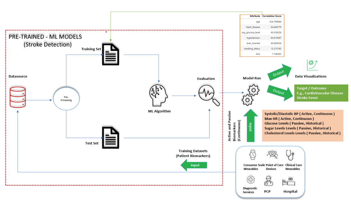
METHODS

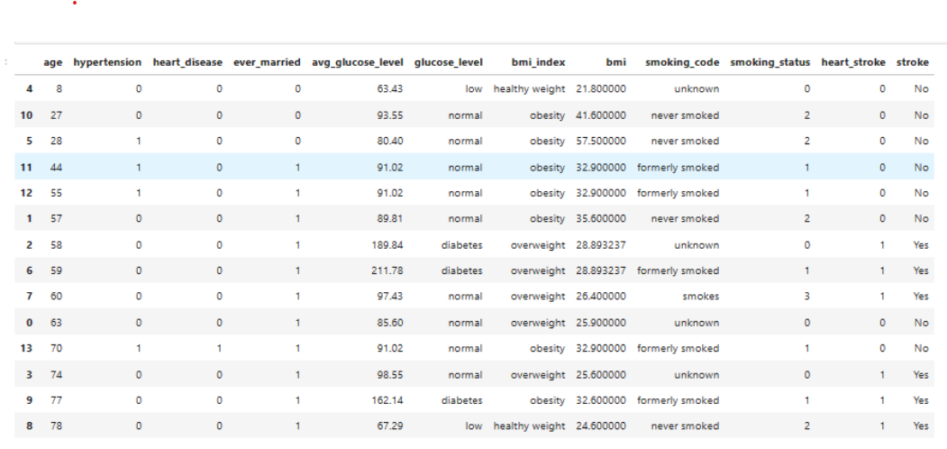
The data sets used to produce results in this presentation were taken from Kaggle. These Kaggle datasets also helped us build conclusions as demonstrated through the following figure below:

Modules

Module	Dataset
Cardiovascular Module	Heart Disease Dataset
Stroke Detection Module	Heart Stroke Dataset

Modeling Process

• I used the programming languages: Python and Panda - for data loading and processing, Matplotlib for data Visualization and sklearn for machine learning and statistical modeling. Also, Jupyter was used as a web-based interactive development environment for developing the models and visualization.
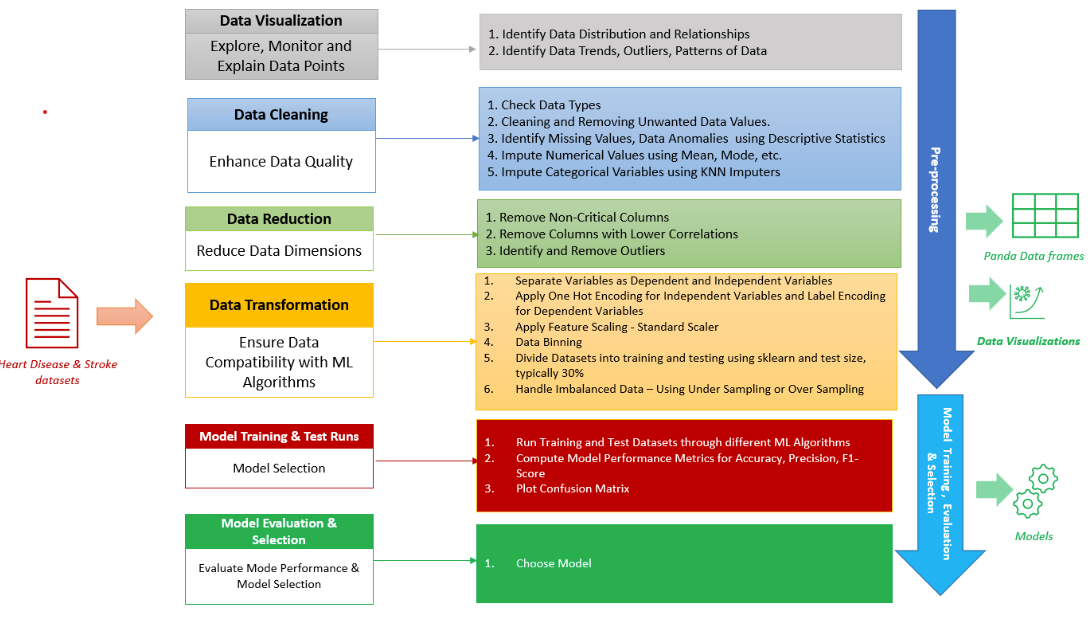
• Machine Learning models are a multi-step process depicted in the below figure:

Modeling Principles

• Many machine learning algorithms fail if the dataset contains missing values.
• You may end up building a biased machine learning model, leading to incorrect results if the missing values are not handled properly.
• Missing data can lead to a lack of precision in the statistical analysis.
• Identify Data Anomalies like features having irrelevant values, like smoking status having ‘unknown’ values.
• Reduce Dimensions by eliminating dimensions that don’t contribute to the target value.
• Remove outliers data to improve accuracy of algorithm.
• Divide datasets into training and testing.
• The Independent Variables are Features that determine the Target Variable need to be at a similar scale and this specifically applies to classification algorithms. Feature Scaling is important for accuracy of distance-based algorithms like KNN, SVM etc. since they are using distances between data points.
• Handle Imbalanced Data, else you would have skewed models that will help detect target output that are biased towards the majority class of features.
• Training Datasets need to be processed via multiple algorithms for determining best performance & accuracy. Also certain models depending on the nature of datasets will be more resilient to data anomalies.

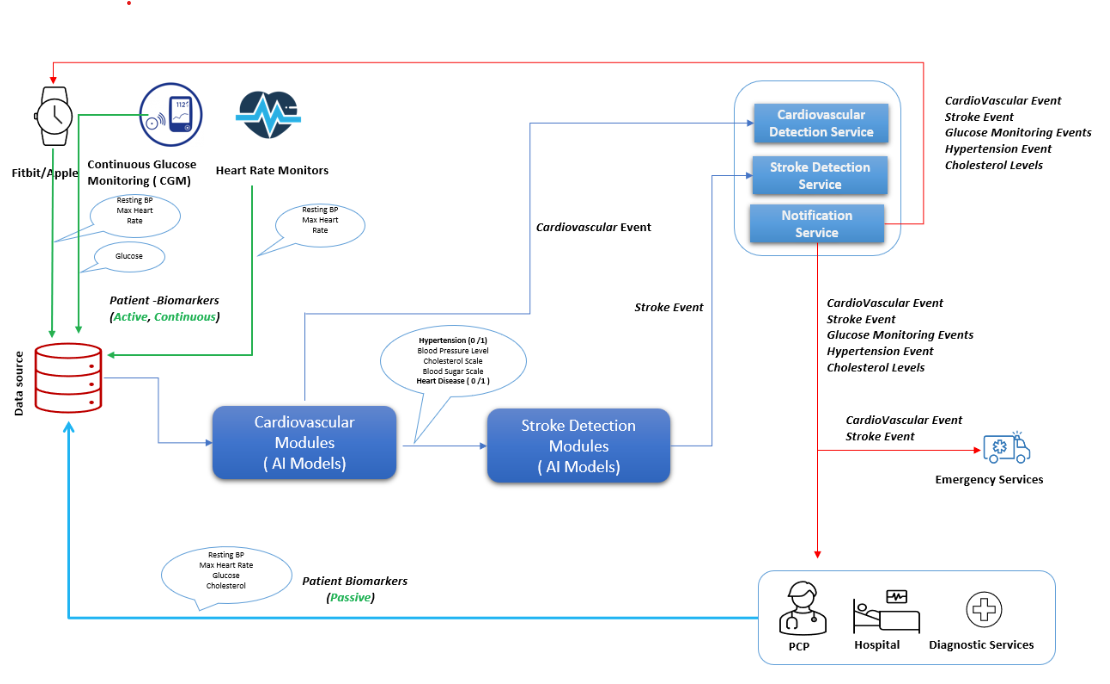
Other technologies used in the Wearable

• CGM(Continuous Glucose Monitoring
• Heart Rate Monitors
• AI Models
• Cardiovascular and Stroke Detection Service
• Notification Service

Pre-processing - Data Cleaning

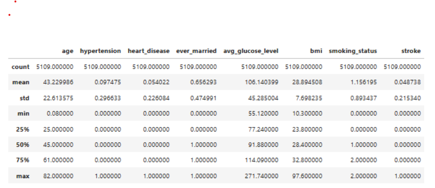
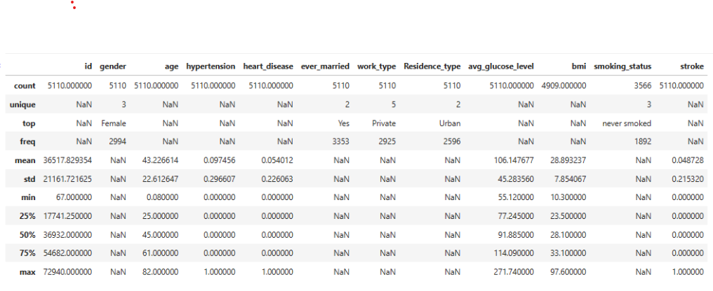
The dataset has 5110 rows. Count indicates 201 bmi null values, 1544 smoking_status with unknown values among the former smokers, never smoked, smokes. The following statistical techniques were used to address missing values & unwanted rows.

• bmi – Typically numerical variables are typically addressed by mean, forwardfill, backward fill techniques. Since 16% of missing bmi values for patients with stroke, is a large population we used mean.
• smoking_status: 30.21% of unknown values of the entire population, 18.8% of unknown values of stroke population. These values cannot be ignored. Categorical Variables are typically addressed by Univariate or Multivariate Analysis. Since there are multiple features that influence stroke occurrence as identified in the Top Correlations, I chose Multi-Variate Analysis. Out of all the techniques tested, LogisticRegression was considered best in terms of accuracy(Handling - Outlier Data as Missing Values through Imputation Methods) for 25% to 75% in the Training/Testing of Datasets.
• gender – one of the rows was labeled other, which is trivial amidst 5110 rows so it was deleted from the row in the panda Dataframe

Pre-Processing - Data Reduction

This step is meant to reduce data dimensions, increase ML Model Performance, and accuracy. The following statistical techniques were applied to the columns.

• Id – a sequence number which does not have any bearing with the Target Feature (stroke) and was removed
• Uses the following categories: age, hypertension, heart_disease, ever_married, avg_glucose_level, bmi, smoking_status
  Steps
  1. Convert the Categorical variables into Numerical variables using Label Encoding for the following categories: gender, ever_married, work_type, residence_type, smoking_status
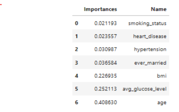
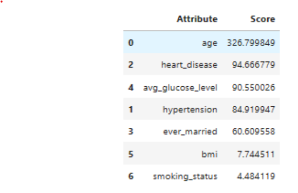
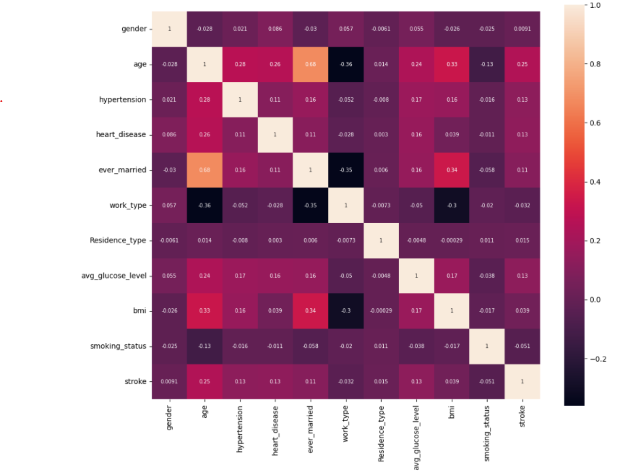
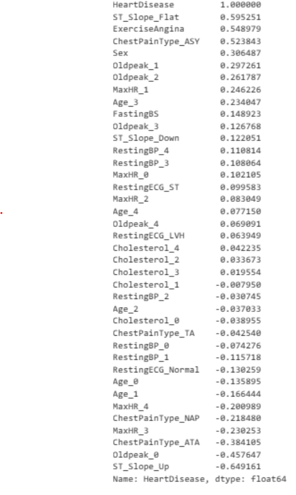
  2. Plotted Correlation Map – indicates a positive correlation with age, hypertension, heart_disease, average_glucose_level with the occurrence of stroke. Hence the following model attributes were removed gender, work_type_residence_type. bmi & smoking_status was one exception, needing further analysis

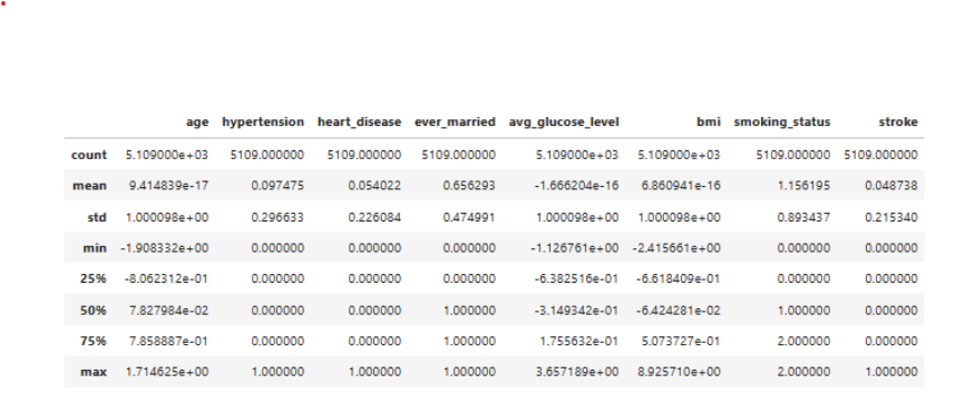
Pre-Processing - Data Scaling

• Supervised and unsupervised learning methods make decisions according to the data sets applied to them and often the algorithms calculate the distance between the data points to make better inferences out of the data. If the values of the features are closer to each other there are chances for the algorithm to get trained well and faster. Apply feature-scaling so that the values scale into similar ranges.
• The pre-scaled data sets the standard deviation of age, avg_glucose_level, and bmi as they are significantly apart from the rest of the values. Therefore, Standard Scaling was applied to the columns

Pre-Processing - Data Transformation (Feature Engineering)

• Compute Effective Correlation to select Model Features
• Apply Encoding
  1. Encode all Independent Variables such as age, hypertension, heart_disease, ever_married, average glucose level, using One Hot Encoding
  2. Encode all Dependent Variables using the technique, LabelEncoding
• Provide Metrics for Imbalance Data. Hence, we use Smote Analysis to balance out the Training Datasets.

Pre-Processing - Data Partitioning

Split datasets into training and testing datasets. We used a 70-30% training / test dataset ratio.

Model Training & Test Runs

• Model training is the most important part of the machine learning process as it results in a working model which will eventually be validated, tested and deployed. The model’s performance during training will determine how well it will work when put into an application for the users. Both the quality of the training data and the choice of the algorithm are central to the model training phase.
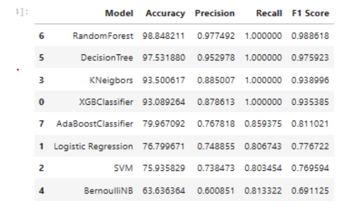
• In most cases, training data is split into two sets for training, validation, and testing. The following models were run through the same training and test datasets to evaluate Model Performance Metrics – Accuracy, Precision, F1-Score, Recall etc. Algorithms differ in accuracy and precision based on the nature of data. So, a number of models were chosen to run through the training and test datasets
• There are two types of Machine Learning Models – Classification and Regression. When the response is binary (only taking two values ex. 0:failure and 1: success) in a Machine Learning model, we use classification models like logistic regression, decision trees, random forest, XGboost, convolutional neural network etc.

Model Evaluation & Selection

• Model evaluation metrics help evaluate the model’s accuracy and measure of performance from this trained model. By using different metrics for performance evaluation, we could improve the overall predictive power of the model before production on unseen data.
• The algorithm, RandomForest has proven to have the best performance and accuracy.
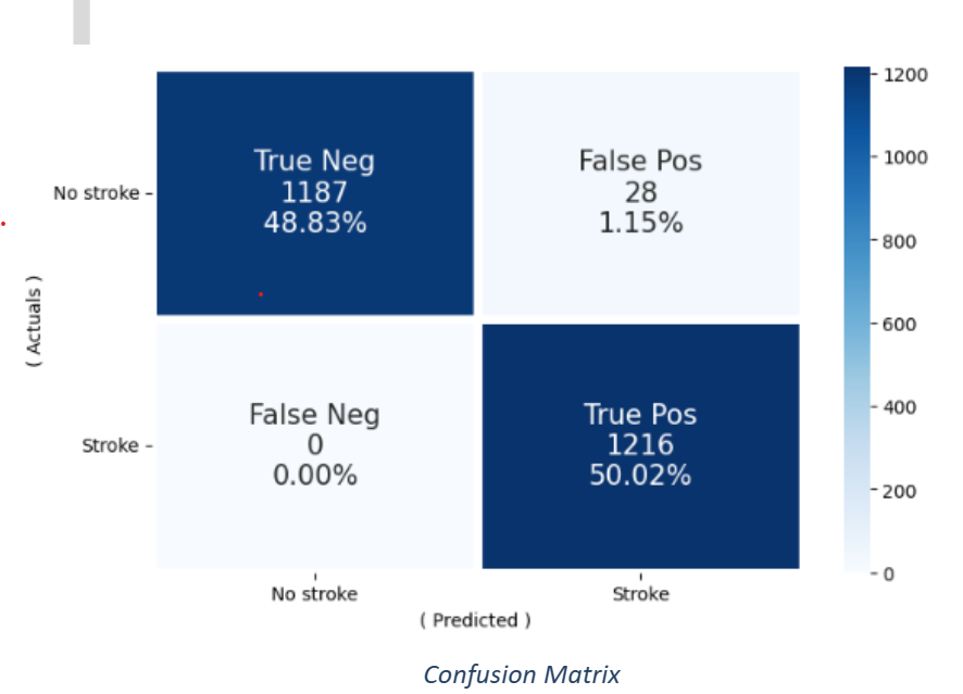
• A confusion matrix is often used to describe the performance of the classification model. This seems to be a good result considering the large number of True Positives. True Negatives are on the lower side because of imbalanced data (4860 patients with No Stroke-0, 249 rows with Stroke-1)

What it means	Class
The predicted values (No Stroke) match the actual value, 919 times	True Positive
The predicted values (Stroke) match the actual value, 6 times	True Negative
The predicted value(No Stroke) doesn’t match the actual value (49) times	False Positive
The predicted value(Stroke Stroke) doesn’t match the actual value (48) times	False Negative

RESULTS

Corelation of Model Parameters

Model Run - Prediction dataset results

Distribution of Model Parameters against Target Variable
( Cardiovascular Disease)

Distribution of Model Parameters against Target Variable
( Stroke Detection)

Problem with this because of Imbalanced Data of Hypertension & HeartDisease for Stroke Occurrence the feature importance appears to the bottom, which is not medically true. We have an explanation of it using statistics in the model code. But Age, Average Glucose Level and bmi are critical features of occurence of heart stroke

Data Scaling / Pre-Scaled datasets

Data Scaling / Post-Scaled datasets

Stroke Detection Accuracy

Confusion Matrix

SOURCE CODE

Machine Learning Models